Dissertation Scribblings I
24/01/2022
If you have done any sort of mechanics in your life, you will have come across something called an energy argument for a problem. This means that basically you can decribe what happens to the energy of a system rather than talking explicitly about the system. For example, if we are considering some system, let us say, a spring with a bob moving in some simple harmonic motion in 1D space. To find an equation to describe the bob in Newtonian Mechanics, we would need to talk about tension in the spring, weight of the bob from it's mass, then the speed of this motion and all these potentially difficult and slightly painful things to measure. An energy argument would use the fact that energy is conserved and assuming there is only two types of energy in this system, potential and kinetic, we can then describe this system just using these two quantities. This leads to an interesting development in mechanics, called the Lagrangian. A Lagrangian is \(\mathcal{L} = K - P\) where \(K\) is the kinetic energy and \(P\) is the potential energy. Moreover, we can describe systems just using Lagrangians, entrant Lagrangian Mechanics.
In Lagrangian Mechanics, what we are interested in is using some set of generalise coordinates to take all of these extra factors from Newtonian Mechanics (Tension, Weight, ...) and almost absorb them so we don't have to worry about specifics, just the general behaviour of the system. This simplifies the whole description and hence we have less equations.
Lie Groups and Algebras
Firstly, we need to get some machinery in order to explain some of those fuzzy concepts clearly. Machinery comes in the form of a group, a specific type of group, the Lie Group. Firstly, a group,
Defintion (Group). A group is a set with a binary operation, \((G, \circ)\) such that,
- There exists an identity, that is there is some \(e \in G\) such that for all \(x \in G\), \(x \circ e = e \circ x = x\)
- There exists an inverse for every element, that is for every \(x \in G\) there is some \(x^{-1} \in G\) such that \(x \circ x^{-1} = x^{-1} \circ x = e\)
- The binary operator, \(\circ\) is associative. That is, for some \(g_1, g_2, g_3 \in G\), \(g_1 \circ (g_2 \circ g_3) = (g_1 \circ g_2) \circ g_3\)
Furthermore, we can define the lie group,
Defintion (Lie Group). A group which has the functions of composition, \(m : G \times G \to G\) defined by \(m(g_1, g_2) = g_1 \circ g_2\) and \(i : G \times G \to G\) defined by \(i(g_1, g_2) = g_1g_2^{-1}\) are smooth.
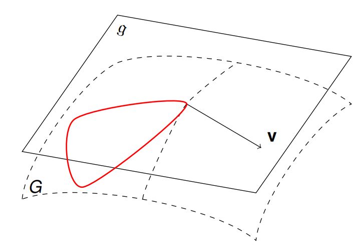
We can think of a Lie Group as a manifold, or a 3D surface. From this 3D surface, we can consider tangent planes to the surface and the planes are made of vectors and these planes are just vector spaces. More formally, these are tangent spaces and a tangent plane at a point \(x \in G\) is denoted by \(T_xM\) assuming that \(M\) is the manifold. Here are two interesting facts, if \(\xi \in T_eG\), then \(g\xi g^{-1} \in T_eG\), hence a tangent space is closed under conjugation action from \(G\) and if \(\xi, \eta \in T_eG\), then \(\xi\eta - \eta\xi \in T_eG\). We note that multiplication isn't necessarily commutative and so \(\xi\eta \ne \eta\xi\) and so we call \(\xi\eta - \eta\xi\) the Lie Bracket and we say that this tangent space is a Lie Algebra as it a vector space endowed with a Lie Bracket, denoted \([\xi, \eta] = \xi\eta - \eta\xi\).
Now on our Lie Groups and Algebras we can talk actions between them. We have two actions we are interested in, one the first variation of the other. The first is the Adjoint, \(\mathrm{Ad} : G \times \mathfrak{g} \to G\), by considering the action by conjugation, \(g \mapsto ghg^{-1}\), it is defined as \(\mathrm{Ad}_g \xi = g\xi g^{-1}\). We can consider the trace pairing, \(\langle A, B \rangle = \mathrm{Tr}(B^TA)\) and now write the coadjoint, \(\langle \mu, \mathrm{Ad}_g\xi \rangle = \langle \mathrm{Ad}^*_g \mu, \xi \rangle\). Now for the second, take the first variation of \(\mathrm{Ad}\), that is, \(\mathrm{Ad}\)\(\mathrm{Ad}\)t.\(\mathrm{Ad}\)ght|{t=0} \(\mathrm{Ad}\){g(t)}\(\mathrm{Ad}\)uite nicely prove this, by doing the following; Let \(g(t) \in G\) where \(g(0) = e\) and \(\dot g(t) = \eta \in T_eG\) $$ \begin{align*} \left.\frac{d}{dt}\right|_{t=0} \mathrm{Ad}_{g(t)}\xi &= \left.\frac{d}{dt}\right|_{t=0} g\xi g^{-1} \\ &= \left[\dot g(t) \xi g^{-1}(t) - g(t)\xi g^{-1}(t)\dot g(t) g^{-1}(t)\right]_{t=0} \\ &= \eta\xi - \xi\eta\\ &= [\eta, \xi] \end{align*}$$
Hence we define \(\mathrm{ad}_g\xi = [\eta, \xi]\) and again we define the coadjoint by \(\langle \mathrm{ad}_g\xi, \mu \rangle = \langle \xi, \mathrm{ad}^*_g\xi\rangle\).
Calculus of Variations (done applied).
A very important idea that we use is called Hamiltons Principle, this says for some Lagrangian, \(\mathcal{L}\), the following holds,
$$ \delta\int_{t_1}^{t_2} \mathcal{L} = 0 $$
This will be our first port of call for proving things, where we call \(\delta\) the first variation and define it as,
$$ \delta f = \left.\frac{d}{dt}\right|_{t=0} f(t) $$
So, if we define a lagrangian in terms of \(g\) and \(\dot g\), as we normally do as usually kinetic and potential energy depend on the position and velocity of the system; then we can start deriving the Euler Legrange Equations,
$$ \delta\int_{t_1}^{t_2} \mathcal{L}(g, \dot g) = \int_{t_1}^{t_2} \left\langle \frac{\partial \mathcal{L}}{\partial R}, \delta R \right\rangle + \left\langle \frac{\partial \mathcal{L}}{\partial \dot R}, \delta R \right\rangle\, dt = 0$$
and then by integrating by parts,
$$ \left.\left\langle \frac{\partial \mathcal{L}}{\partial R}, \delta R \right\rangle\right|_{t_2} + \left.\left\langle \frac{\partial \mathcal{L}}{\partial \dot R}, \delta R \right\rangle\right|_{t_1} + \int_{t_1}^{t_2} \left\langle \frac{\partial \mathcal{L}}{\partial R} - \frac{d}{dt}\frac{\partial \mathcal{L}}{\partial \dot R}, \delta R \right\rangle = 0$$
and we set boundary conditions, to say at \(t_1\) and \(t_2\) is just zero. Hence we get that,
$$ \int_{t_1}^{t_2} \left\langle \frac{\partial \mathcal{L}}{\partial R} - \frac{d}{dt}\frac{\partial \mathcal{L}}{\partial \dot R}, \delta R \right\rangle = 0$$
and so we can derive the Euler Lagrange Equations,
$$ \frac{\partial \mathcal{L}}{\partial R} - \frac{d}{dt}\frac{\partial \mathcal{L}}{\partial R} = 0 $$
These describe the first way we can use Geometric Mechanics (adjacent mathematics) to describe real world systems. Let us now take an example, the spherical pendulum,
Firsty, let \(K = \frac{1}{2}mv^2 \) and we are interested in how we can represent \(v\) in terms of our coordinated. We can do it through this equation, \(v = \sqrt{\dot x^2 + \dot y^2 + \dot z^2}\). We can plug in and differentiate and find that \(K = \frac{1}{2}mR^2 \left( \dot \theta + \dot \phi^2\sin^2\phi\right)\). Our system also one has one potential, gravitational and so \(P = -mgz = -mgR(1 - \cos \theta)\) and so our Lagrangian is,
If we now differentiate this Lagrangian by each basis vector as implied above, we get,
and these are the Euler-Lagrange Equations for the pendulum. I shall leave this here, for now, but next time, hopefully we can work towards doing this for the Euler-Poincare equations and then move onto Euler-Poincare Reduction.